


15 Apr Climate Projection Table

Global temperature anomaly projections beyond 2024 based on historical data
In 1856 Eunice Newton Foote, an amateur scientist from upstate New York, suggested: An atmosphere of that gas [carbon dioxide] would give to our earth a high temperature; and if as some suppose, at one period of its history the air had mixed with it a larger proportion than at present, an increased temperature from its own action as well as from increased weight must have necessarily resulted.
In effect, CO2 and other greenhouse gases (GHGs) would trap heat transmitted from Earth, upset its energy equilibrium and initiate global warming. Her predictions were soon confirmed by European scientists, including Svante Arrhenius, who in 1896 developed a theoretical model linking increased CO2 levels from fossil fuel combustion to potential global warming. He calculated that doubling atmospheric CO2 concentration [CO₂] would result in an increase in Earth’s average surface temperature of approximately 5–6°C.
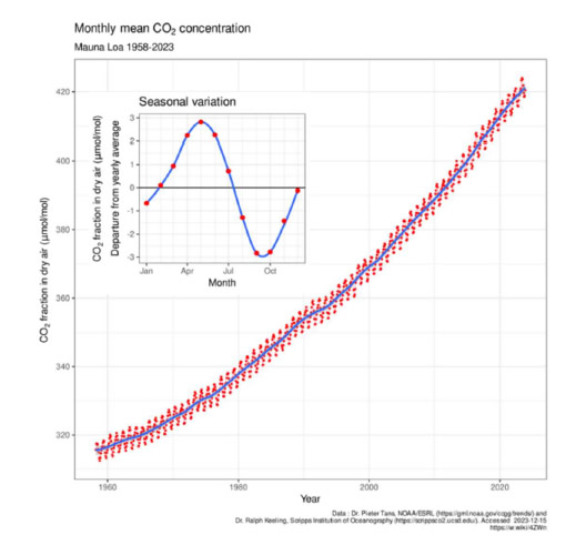
Charles David Keeling made it possible to test these theories in 1958 by initiating daily measurements of ( [CO₂] ) from an observatory atop a 3500-metre-high volcano on Mauna Loa in the Pacific Ocean. His records have enabled the NOAA Global Monitoring Laboratory to analyse ice cores to create an historical [CO₂] record back to 800,000 BCE1. A small portion of this data set has supplied the [CO2] data used to create Figure 1.2.
The other half of the equation, the global temperature anomaly ΔT, has been derived from data sets published by the Met Office Hadley Centre in England. Global temperatures have been recorded continuously at various observatories around the world ever since Thomas Hornsby, mathematician and astronomer, established what is now known as the Met Office Hadley Centre in 1772. Others followed, the Prague Klementinum began recording in 1775, the Sydney Observatory in 1859 and the Central Park weather station in New York in 1869. These data and others are now regularly processed by the Met Office Hadley Centre who issue a ‘Global average temperature anomaly relative to 1861-1890’ every three months and this is the source for ΔT adopted for this study3. ΔT is the global average temperature anomaly relative to 1861-1890 and is the difference in average land-sea surface temperature compared to the 1861-1890 mean which was about 14oC. Since the industrial revolution Earth’s average surface temperature has increased by ΔT, currently about 1.48oC.
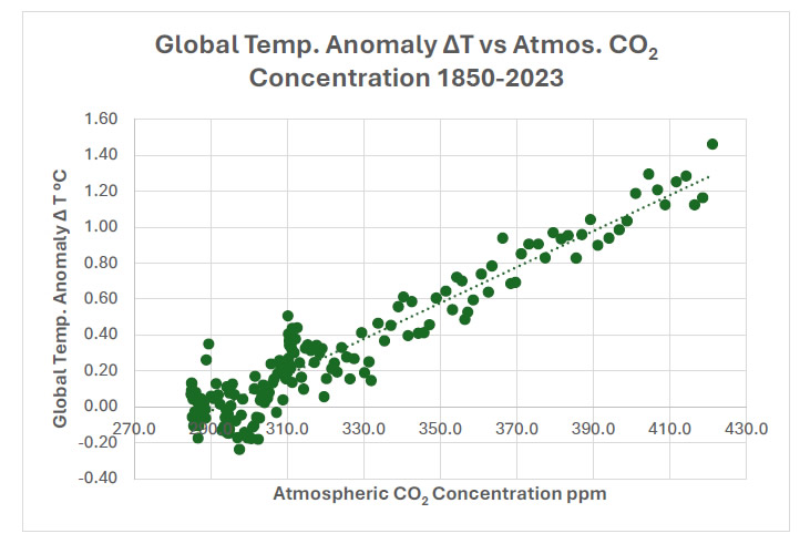
Figure 1.2 demonstrates a strong correlation between [CO2] and ΔT at the rate of 0.010oC/ppm CO2. At this rate a doubling of CO2 concentration from 285 to 570 will result in a 2.85oC rise in ΔT. As mentioned earlier, Svante Arrhenius calculated that doubling CO2 would result in an increase in Earth’s average surface temperature of approximately 5–6°C. Melting ice is the likely explanation for this discrepancy. In Slater et al., 2021, Earth’s ice imbalance 4 it is estimated ~0.028 Tt (trillion tonnes) of ice have been lost since 1970. This would have consumed enough latent heat to increase ΔT 1.83oC which accounts for much of the dfference between Arrhenius’s 6oC and the projected 2.85oC from Figure 1.2. Fortunately, the ice lost to date is only a tiny fraction of the whole ~27.2 Tt (trillion tonnes) so the linear relationship between CO2
concentration and global temperatures should endure until there are practical ways to rein in the use of fossil fuels for manufacturing, power generation, agriculture, transport and air-conditioning.
The Paris Agreement signed by delegates to the 21st Conference of the Parties (COP21) to the United Nations Framework Convention on Climate Change (UNFCCC) in Paris in December 2015 provides targets for this endeavour. The agreement binds the 197 signatories to the agreement
- to limit global temperature increase to well below 2 degrees Celsius above preindustrial levels.
- to pursue efforts to limit the temperature increase to 1.5 degrees Celsius above pre-industrial levels.
- to reduce greenhouse gas emissions to achieve a balance between anthropogenic emissions by sources and removals by sinks of greenhouse gases in the second half of this century (net zero emissions).
- to prepare, communicate and maintain successive Nationally Determined Contributions (NDCs) that individual countries intend to achieve.
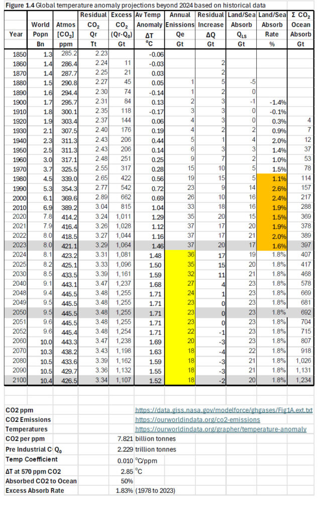
As a basic tool to plan and monitor these fforts on a global scale, Figure 1.3 is a spreadsheet analysis of historical records that allows them to be projected forward from 2023. The underlying principle for the analysis of past records and the forward projections is that global warming is caused by the atmospheric greenhouse effect. CO₂ is a greenhouse gas. It absorbs and re-emits infrared radiation, trapping heat in the Earth’s atmosphere. Excess CO₂ traps more heat disrupting the balance between incoming solar radiation and outgoing infrared radiation. This energy imbalance causes global surface warming, ocean heat uptake, melting ice sheets, rising sea levels and changes in weather patterns. Each of these effects can be observed, the most obvious being global surface warming (see Figure 1.2) and melting ice sheets.
Between the end of the last Ice Age (~11,700 years ago) and the start of the industrial revolution, say 1850, Earth’s climate was stable save for minor natural fluctuations. [CO2] was 285 ppm equivalent to a baseline atmospheric CO2 quantity, Q0 of 2.229 trillion tonnes. ΔT was zero. The first step in analysing historical carbon dioxide emission destinations from that time on is the creation of an accurate historical record of CO2 emissions.
This involves a combination of statistical reporting, fuel consumption data, industrial activity records, and satellite measurements. The process begins with national and sectoral data on fossil fuel use coal, oil, and natural gas— ollected by governments and energy agencies. Emissions from cement production, land use changes, and deforestation are also estimated using activity data and scientific models. These figures are then converted into carbon dioxide equivalents using standardized emissions factors. Independent scientific institutions, such as the Global Carbon Project, aggregate and verify this information to produce consistent global estimates. Increasingly, satellite-based atmospheric observations and machine learning techniques are used to cross-check and refine the accuracy of reported emissions, particularly in regions with limited transparency. The result is a comprehensive yearly snapshot of how much CO₂ humanity adds to the atmosphere. The record adopted for the compilation of Figure 1.3, ‘Global temperature anomaly beyond 2024 based on projected global CO2 emissions’ is published by Our World in Data5.
There is now sufficient data to compile the table up to 2023. Residual CO2 in the atmosphere in trillion tonnes, Qr, is simply [CO2] multiplied by 7.821/1000. Excess CO2 in the atmosphere in billion tonnes is (Qr-Q0)*1000. The annual residual CO2 increase in the atmosphere ΔQ is simply the increase in Qr from one year to the next in billion tonnes.
The CO2 emissions that do not remain in the atmosphere are absorbed by land and sea in what are known as the terrestrial and marine carbon sinks. Plants absorb CO₂ from the air and use it to produce sugars via photosynthesis. Forests, grasslands, and crops are major carbon absorbers, especially tropical and temperate forests. CO₂ from the atmosphere dissolves into the ocean surface. Tiny plankton in the ocean’s surface absorb CO₂ during photosynthesis. When these organisms die, the carbon in their bodies sinks into the deep ocean, sequestering it for centuries or more. CO₂ reacts with seawater to form bicarbonate (HCO₃⁻) and carbonate ions (CO₃²⁻). This buffering system allows the ocean to store vast amounts of carbon although it also leads to ocean acidification.
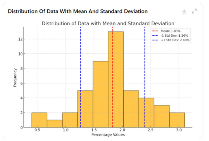
QLS, the CO2 absorbed by land and sea is simply the difference between annual emissions Qe and the annual residual CO2 increase in the atmosphere ΔQ. The ice records show that [CO2] began to grow around 1880 when it had reached 290 ppm. An examination of the historical records show that it took around 100 years for the carbon dioxide cycle to stabilise but when it did it became clear that the annual land sea absorption rate fell into a band between 1.3 and 2.4% of the excess CO2 in the atmosphere (Qr-Q0) with a mean of 1.83% as per Figure 1.3.
This land/sea absorption factor of 1.83% can now be used to project [CO2], Qr ΔT and ΣQs forward from an adopted future emissions profile. Referring to Figure 1.4, the year 2024 can be used as an example. To be optimistic it will be assumed that Qe2024 is 36 Gt.
QLS2024 is assumed to be 1.83% of the excess atmospheric CO2 for 2023 i.e. 19 Gt. This leaves ΔQ2024 as 20Gt and from this it’s a simple process to calculate the remaining elements of the 2024 row and so on to 2100.
Figure 1.4, Global temperature anomaly projections beyond 2024 based on historical data6,7,8,9,10 is based on an emissions scenario that assumes annual emissions peak in 2023 at 37 Gt and drop to 36 Gt in 2024 from where it steadily reduces to 23 Gt in 2050 to achieve net zero and 18 Gt in 2100 to bring ΔT back to 1.52oC.
List of abbreviations and symbols
a albedo
AAAS American Association for the Advancement of Science
AR6 Assessment report 6
Bn billion
[CO₂] atmospheric CO2 concentration
CCA Climate Change Authority
CFC chlorofluorocarbon
CH4 methane
CO2 carbon dioxide
CO₃²⁻ carbonate
CMIP6 Coupled Model Intercomparison Project Phase 6
COP21 Conference of the Parties UNFCCC Paris 2015
COP26 Conference of the Parties UNFCCC Glasgow 2023
CPRS Carbon Pollution Reduction Scheme
oC degrees Celsius
FAR first assessment report
g/mol grams per mole
GHG greenhouse gas
Gt gigatonne, billion tonnes
GW gigawatt
H⁺ hydrogen ion
H2O water
HCO3- bicarbonate
IPCC Intergovernmental Panel on Climate Change
K degrees kelvin
kW kilowatt
kWh kilowatt hour
MW megawatt
MWh megawatt hour
Mt megatonne, million tonnes
NDC Nationally Determined Contribution
PhD Doctor of Philosophy
ppm parts per million
S the solar constant (approximately 1367 W/m²)
SO2 sulphur dioxide
TWh terawatt hour
Tt teratonne, trillion tonnes
UN United Nations
UNFCCC United Nations Framework Convention on Climate Change
USA United States of America
UV ultraviolet
W/m2 watts per square metre
WMO World Meteorological Organization
ΔT global average temperature anomaly relative to 1861-1890
1 NOAA Global Monitoring Laboratory – Trends in Atmospheric Carbon Dioxide (2025); EPA based on various sources (2022) – with major processing by Our World in Data
2 Monthly mean CO2 concentration, Mauna Loa 1958–2023, Dr Pieter Tans NOAA/ESRL, Dr Ralph Keeling, Scripps Institution of Oceanography.
https://commons.wikimedia.org/wiki/Template:Other_versions/Mauna_Loa_CO2_monthly_mean_concentration . Accessed 15 December 2023.
3 Met Office Hadley Centre – HadCRUT5 (2025) – with major processing by Our World in Data. “Global average temperature anomaly relative to 1861-1890” [dataset]. Met Office Hadley Centre, “HadCRUT5 HadCRUT.5.0.2.0” [original data].
4 Slater, T., Lawrence, I. R., Otosaka, I. N., Shepherd, A., Gourmelen, N., Jakob, L., Tepes, P., Gilbert, L., and Nienow, P.: Review article: Earth’s ice imbalance, The Cryosphere, 15, 233–246, https://doi.org/10.5194/tc-15-233-2021, 2021.
5 Ritchie, Hannah; and Max Roser. ‘CO₂ Emissi
6 Ritchie, Hannah, and Roser, Max. ‘Population over the Long Run with Projections.’ Our World in Data. https://ourworldindata.org/grapher/population-long-run-with-projections?country=~OWID_WRL. Accessed 18 December 2024.
7 Ritchie, Hannah, and Roser, Max. ‘Population over the Long Run with Projections.’ Our World in Data. https://ourworldindata.org/grapher/population-long-run-with-projections?country=~OWID_WRL. Accessed 18 December 2024.
8 Monthly mean CO2 concentration, Mauna Loa 1958–2023, Dr Pieter Tans NOAA/ESRL, Dr Ralph Keeling, Scripps Institution of Oceanography. https://commons.wikimedia.org/wiki/Template:Other_versions/Mauna_Loa_CO2_monthly_mean_concentration . Accessed 15 December 2023.
9 Ritchie, Hannah; and Roser, Max. ‘Temperature Anomaly.’ Our World in Data, https://ourworldindata.org/grapher/temperature-anomaly. Accessed 18 December 2024.
10 Ritchie, Hannah; and Max Roser. ‘CO₂ Emissions.’ Our World in Data, https://ourworldindata.org/co2-emissions. Accessed 18 December 2024.
Nicola Fleming
Posted at 13:44h, 30 AprilGreat article David!